
Indexed Access To Cansim Series In R
In this example, we will use the cansim package to access gender-specific data by vector from Statistics Canada’s NDM using the cansim package from Mountain Math.
Packages USED
The key package used in this vignette is the cansim package which accesses vectors, in this case, from the NDM database of Statistics Canada. Key packages include
- Dplyr/tidyverse – for processing the tibble
- ggplot2 – part of tidyverse for plotting the results
- cansim – package to access data using the NDM api.[1]
Project Outline
NDM product tables (aka CANSIM) can be retrieved with a wealth of classification or META data as well as the coordinate. The latter provides a superlative index into the structure of the table. One of the challenges with many tables is that they contain more information than required for a particular project in terms of both data observations and detail of vectors. The retrieval can be simplified by just retrieving vectors for specific observations. However, the challenge is to easily and flexibly select vectors. The coordinate identifier and associated meta data can be used to select series. This allows the creation of scripts in which the series can be appropriately organized by concept (gender, province etc) and for the time range required. This can result in a substantial increment in speed and more importantly provide a structured organization to the retrieval. The latter facilitates the use of the more power features of tidyverse.
This note documents two scripts:
1)one-time retrieval of full table and creation of an index file which is simply the last observation of the table.
2)Retrieve required v numbers and observations to plot the change in employment rates since a particular period of time.
Script 2 is much more efficient to run and re-run because only a portion of the time series and observations are retrieved.
In corporate environments, it may be necessary to use a proxy setting. This is documented in the citation for the cansim package above.
All scripts will be available in the download section. https://www.jacobsonconsulting.com/index.php/downloads-2/indexed-access-to-ndm-series-in-r/download
Developing the Index File
This script is quite simple. The table is retrieved and saved as an RDS file (not really needed in this case). After retrieval, the table is filtered for the last observation only and saved as an RDS file with an appropriate file name.
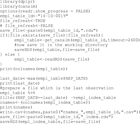
The original table from the retrieval need not be saved. The index file includes all the columns such as value and date for reference purposes. A csv file of the column names is saved for documentation.
Employment Rates
The base table used for this analysis contains significant detail by age and employment type. Because we want to show employment rates for full- and part-time workers, we must calculate employment rates on the fly as the ratio of employment to source population. The first script segment defines the packages used and retrieves the index table using readRDS, the reverse of the command used to save it above.

The next segment unpacks the index table to separate the coordinate into addressable single indexes, Columns that are not required are also dropped.

The columns of the coordinate are renamed to useful variable names. These will be used to select the vectors required. This is much easier than trying to select by the text variables in the basic table. The latter are matched to the coordinate codes to provide a mapping for use in selecting text entries and other documentation. Because we do not want to show all levels of education attainment, the education table is extended to include an aggregation variable, “edtype”. This will be used to collapse employment and population.
The values used to select the series are determined by examining the tables created above.

The code segment above defines some key parameters and selects and aggregates the source. Population by summarizing over the “edtype” variable. Note that the variables from the index table are joined with the data required from NDM so that the full attribute set is available.
The next set of code starts the main loop. Looping is over labour force type (full- and part-time), gender and time.

The next set of code prepares the basic analytical rates by joining the tibble retrieved above with the population tibble after appropriate aggregation. Note that the population tibble is joined using all the relevant classification variables. We are calculating year over year growth rates but also growth rates from February 2020. The code was originally set up to process the current and preceding months.
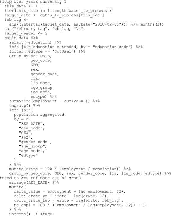
The next segment calculates shares of change and employment for analytical purposes.

Charts for four displays are planned. After setting up the parameters, the basic data is adjusted to select the date to plot, the gender and to copy the variable to plot to a specific variable in the data set that can be referenced in the ggplot2 package. The “.data” element is referred to as a pronoun in the tidyverse programming documentation. The reference is https://dplyr.tidyverse.org/articles/programming.html.

The next code segment uses plot_data_2 in ggplot with the parameters defined above to characterize the chart.

Note that the plot_value variable is used to position the text label above the actual bar.
The final code segment saves each plot as a separate png and builds up a list of pngs which is saved for subsequent processing into a PDF or other report.

[1] https://www.rdocumentation.org/packages/cansim
1) one-time retrieval of full table and creation of an index file which is simply the last observation of the table.
2) Retrieve required v numbers and observations to plot the change in employment rates since a particular period of time.