A Tidyverse Example for NDM Vector Processing
This section examines a simple script to process a seven series downloaded from the NDM vector search facility. The script reads the data and analyzes the contents. The data are then reordered by time and converted from the tall narrow format of the data as retrieved to a wide csv with time in columns. Percentage changes are calculated for selected series. A plot of one series is done. Selected series are also annualized using averages. This script was developed to highlight features of the Tidyverse for processing data into a useful form. Normally, all analysis should be done in R rather than export to older technologies such as Excel. However, in this case, the script was developed to show how to port data to CSVs useable by Excel. The full script with comments is included as Appendix A and a log file as Appendix B in the accompanying pdf in the R notes downloads..
The initial set of code sets the working folder or directory and loads the required package libraries for this simple project. The backslashes are duplicated because the backslash is an “escape” character that signals special processing of the subsequent character.
setwd( "D:\\OneDrive\\ndm_r_runs") library(tidyverse) library(lubridate)
The next set of code reads the data in using the readr routine read_csv.
input_file<-"vectorsSearchResultsNoSymbols.csv" input_data<-read_csv(input_file) print(colnames(input_data))
The print statement will show that the column names in the input_data data frame include "Vector", "Frequency", "Description", "Reference Period", "Unit of Measure", "Value" and "Source". In the discussion below, each column is considered a variable in the data frame.
One of the key features in modern R is the use of the pipe (%>%). This “pipes” the results from one command to the next and facilitates the linkage of commands without unnecessary results.
The next commands create a series directory by selecting unique or distinct values for the Vector and Description variables. The results are then printed.
series_directory<-select(input_data,c("Vector","Description"))%>%distinct()
print(series_directory)
One challenge with data retrieved from NDM is that the sort may not be optimal. For time series, most users want high to low. The other challenge is that the representation of the time period is not normal in that a day is not including with the month. Excel automatically converts Month Year combinations to dates including the first day of the month. The next command mutates the input data set to include two new variables, obs_date and obs_year. The date variable is created by pasting the string “1 “ to each reference period entry and then converting to system standard dates using the day-month-year function (dmy) from the lubridate package.
input_data<-mutate(input_data,obs_date=
dmy(paste0("1",
input_data$"Reference Period",sep="")),
obs_year=year(obs_date))
It should be noted that variable columns in a data frame are referenced by using the data frame name concatenated with the $ sign to the variable name. Variable names with embedded blanks must be enclosed in quotes.
The next command creates a sorted data frame by vector and date, mutates it to include the variable obs_pch which is the percentage change and filters the data to include only data from 2015 forward.
sorted_data<-arrange(input_data,Vector,obs_date)%>%
mutate(obs_pch=((Value/lag(Value,1))-1)*100)%>%filter(obs_year>=2015)
The sorted_data data frame is still a tall data frame with one value observation per row. The next command set creates a value_spread data frame with the vector number, the description and a new variable Type indicating that the data are untransformed. The data are spread into a wide data set with one column for each month in obs_date.
value_spread<-select(sorted_data,Vector, Description,
obs_date,Value)%>%mutate(Type="Raw")%>%
spread(obs_date,Value)
Note that in R, the capitalization of all variables is critical. In other words, to be found, Description must be capitalized.
We want to add percentage change data to the analysis. However, the vectors chosen for this run include 3 vectors from the Bank of Canada’s price series which are already in change format. Therefore, they should be excluded from the calculation. This is done by excluding all rows with vector names in a list defined from the 3 Bank series.
boc_series<-c("V108785713", "V108785714", "V108785715")
pch_spread<-select(sorted_data,Vector,Description,obs_date,obs_pch)%>%
mutate(Type="PCH")%>%
filter(!(Vector %in% boc_series))%>%
spread(obs_date,obs_pch)
The filter command uses the logical not (!) to exclude vectors in the list of bank series.
The final two commands concatenates the two frames by row using the rbind command and writes the resulting output data frame to a CSV file.
output_data<-rbind(value_spread,pch_spread)
write.csv(output_data,file="Vector_output_data.csv")
The first columns of the resulting data set are shown below.
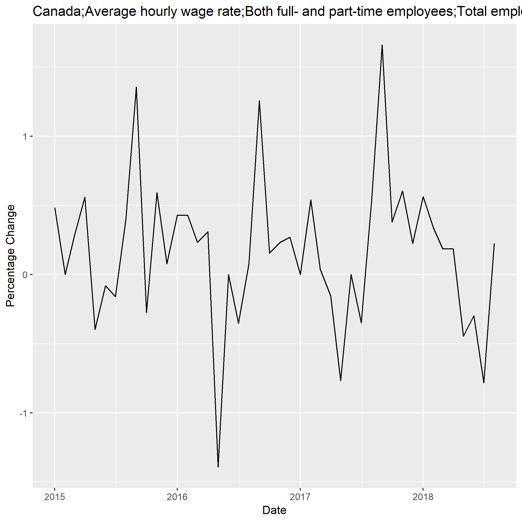
Just to show that one can do some work in R, the next lines select and plot the labour force average hourly wage rate. The resulting chart is saved as PNG file. The chart title is extracted from the series directory created above.
plot_series<-"V2132579"
chart_title=select(series_directory,Vector,Description)%>%filter(Vector==plot_series)
plot_data<-select(sorted_data,Vector,obs_date,obs_pch)%>%filter(Vector==plot_series)
plot1<-ggplot(plot_data,aes(x=obs_date,y=obs_pch))+geom_line()+
labs(title=chart_title$Description,x="Date",y="Percentage Change")
ggsave(plot1,file=paste0(plot_series,"_percentage_change.png"))
The resulting graph is show below. It uses basic defaults.

The final task in this simple script is to create an annualized data set. This means to take the annual average of all series. However, the labour force wage rate is excluding because correct annualization requires weighting by monthly employment which is not available in the data set.
lfs_series<-"V2132579"
annual_spread<-select(sorted_data,Vector,Description,obs_year,Value)%>%
filter(!Vector==lfs_series)%>%
group_by(Vector,Description,obs_year)%>%
summarize(Value=mean(Value))%>%
mutate(Type="Annual Average")%>%
spread(obs_year,Value)
write.csv(annual_spread,file="Annualized_vector_data.csv")
In this section of code, the key verb is the group_by command which sets the limits for which the mean or average calculation is applied (by year) and includes unique copies of the Vector and Description in the output data set before spreading it by year.
The resulting data set is shown below.

